Create a machine learning model that predicts whether an individual has an income of over $50K. Perform a fairness audit in order to assess whether or not the algorithm displays bias with respect to sex.
Author
Katie Macalintal
Published
March 29, 2023
Auditing Allocative Bias
In this blog post, we are going to train a machine learning model to predict whether an individual in the state of New Jersey (NJ) has an income of over $50K based on demographic characteristics, excluding sex. After training this model, we will perform a fairness audit to assess whether or not our model displays bias with respect to sex.
Preparing the data
We first download the PUMS data for the state of New Jersey and add a column to indicate whether the individual makes more than $50K. This new column is titled SAL50K and has the value 1 if the individual makes $50K or more and 0 otherwise.
from folktables import ACSDataSource, ACSEmployment, BasicProblem, adult_filterimport numpy as npSTATE ="NJ"data_source = ACSDataSource(survey_year='2018', horizon='1-Year', survey='person')# Download PUMS data for NEW JERSEY acs_data = data_source.get_data(states=[STATE], download=True)# Add column to indicate whether individual makes more than 50K acs_data = acs_data.assign(SAL50K =1* (acs_data['PINCP'] >=50000))acs_data.head()
RT
SERIALNO
DIVISION
SPORDER
PUMA
REGION
ST
ADJINC
PWGTP
AGEP
...
PWGTP72
PWGTP73
PWGTP74
PWGTP75
PWGTP76
PWGTP77
PWGTP78
PWGTP79
PWGTP80
SAL50K
0
P
2018GQ0000003
2
1
2302
1
34
1013097
12
23
...
3
12
2
3
14
12
13
12
2
0
1
P
2018GQ0000017
2
1
1800
1
34
1013097
11
51
...
2
9
9
19
10
19
19
2
10
0
2
P
2018GQ0000122
2
1
2104
1
34
1013097
24
69
...
22
45
2
3
24
24
23
44
1
0
3
P
2018GQ0000131
2
1
800
1
34
1013097
90
18
...
96
158
96
14
145
157
15
88
156
0
4
P
2018GQ0000134
2
1
1700
1
34
1013097
68
89
...
67
68
69
6
123
131
132
127
68
0
5 rows × 287 columns
Based on the dimensions of our downloaded PUMS data, we see that there are over 250 features documented. These are too many features to train on, so in our modeling tasks, we will only focus on …
AGEP is age
SCHL is educational attainment
MAR is marital status
RELP is relationship
CIT is citizenship status.
MIG is mobility status
MIL is miliary service
ANC is ancestry recode
RAC1P is race (1 for White Alone, 2 for Black/African American alone, 3 for Native American alone, 4 for Alaska Native alone, 5 for Native American and Alaska Native tribes specified, 6 for Asian alone, 7 for Native Hawaiian and Other Pacific Islander alone, 8 for Some Other Race alone, 9 for Two or more races)
ESR is employment status (1 if employed, 0 if not)
DIS, DEAR, DEYE, and DREM relate to certain disability statuses
Note that we do not include …
SEX is binary sex (1 for male, 2 for female)
SAL50K is added column indicating whether the individual makes more than 50K
for SEX is our group choice that we will evaluate bias against and SAL50K is our target variable.
# Possible features suggested to usepossible_features=['AGEP', 'SCHL', 'MAR', 'RELP', 'DIS', 'ESP', 'CIT', 'MIG', 'MIL', 'ANC', 'NATIVITY', 'DEAR', 'DEYE', 'DREM', 'SEX', 'RAC1P', 'ESR', 'SAL50K']# Subset features want to usefeatures_to_use = [f for f in possible_features if f notin ["SEX", "PINCP", "SAL50K"]]acs_data[features_to_use].head()
AGEP
SCHL
MAR
RELP
DIS
ESP
CIT
MIG
MIL
ANC
NATIVITY
DEAR
DEYE
DREM
RAC1P
ESR
0
23
21.0
5
17
2
NaN
5
2.0
4.0
1
2
2
2
2.0
6
6.0
1
51
20.0
4
17
2
NaN
4
1.0
4.0
1
2
2
2
2.0
1
1.0
2
69
19.0
3
16
1
NaN
1
1.0
4.0
4
1
2
2
2.0
1
6.0
3
18
16.0
5
16
1
NaN
1
1.0
4.0
2
1
2
2
1.0
9
6.0
4
89
19.0
2
16
1
NaN
1
1.0
4.0
4
1
2
2
1.0
1
6.0
Now that we have chosen our features to use, we construct a BasicProblem that allows us to use these features to predict whether an individual makes more than $50K using the SEX as the group label. Doing this gives us our feature matrix features, our label vector label, and group label vector group.
Based on the dimensions of our df data frame, which holds all the feature values for every individual in our training data, we see that our training data has information for about 70868 different individuals.
Based on the table below, we see that only about 31.21% of the individuals in our training data make more than $50K.
Based on the table below, we see that of those who make more than $50K in our training data, about 59% of them are male while the remaining 41% of them are female.
Overall, based on these tables it looks like males are more likely to make more than $50K.
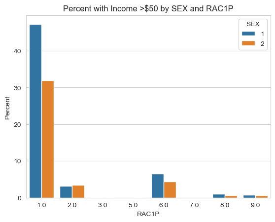
We can also inspect intersectional trends by studying the proportion of those who make more than $50K broken out by both our chosen group labels of SEX and an additional group label. Here we have chosen to use RAC1P.
We first create a data frame that holds that information and then use seaborn package to visualize the new data frame.
Remember that …
RAC1P is race (1 for White Alone, 2 for Black/African American alone, 3 for Native American alone, 4 for Alaska Native alone, 5 for Native American and Alaska Native tribes specified, 6 for Asian alone, 7 for Native Hawaiian and Other Pacific Islander alone, 8 for Some Other Race alone, 9 for Two or more races)
SEX is binary sex (1 for male, 2 for female)
import seaborn as sns# Create new dataframefiltered_df = df[df['>50K'] ==1]intersectionality = filtered_df.groupby(['SEX', 'RAC1P']).size().reset_index(name='count')intersectionality['Percent'] = (intersectionality['count'] /len(filtered_df.index) *100).round(2)# Visualize it using seaborn packagesns.set_style("whitegrid")sns.barplot(x="RAC1P", y="Percent", hue="SEX", data=intersectionality).set(title='Percent with Income >$50 by SEX and RAC1P')
[Text(0.5, 1.0, 'Percent with Income >$50 by SEX and RAC1P')]
Based on the bar plot above, we see that white men make up the majority of those who make more than $50K in our data, followed by white women. In our training data, we also see that individuals who are not white, regardless of their sex, make up a small portion of those who make more than $50K.
Training Our Model
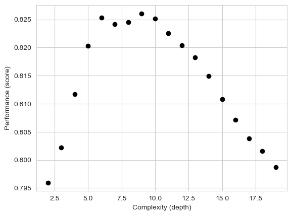
Now it is time to train our model. The model we chose to use is the DecisionTreeClassifier, which requires a specified max_depth. To find our optimum max_depth we use cross validation.
In a Jupyter environment, please rerun this cell to show the HTML representation or trust the notebook. On GitHub, the HTML representation is unable to render, please try loading this page with nbviewer.org.
Now that our model is trained, we can audit how it does on the test data. We first define a function that may help with finding the positive predictive values (PPV), which is the proportion of positive results that are truly positive, the false negative rate (FNR), and false positive rate (FPR). We also extract our predictions y_hat on the test data.
We can also examine the accuracy, PPV, FNR, and FPR for each subgroup in our test data. So examining group 1, is equivalent to examining these values for the males in the test data. And exmaining group 2, is equivalent to examining these values for the females in the test data.
# Accuracy for men(y_hat == y_test)[group_test ==1].mean()
0.8259855376720318
# Accuracy for women (y_hat == y_test)[group_test ==2].mean()
0.8167104111986002
#PPV FNR and FPR for malefind_PPV_FNR_FPR(y_test[group_test ==1], y_hat[group_test ==1])
We see that the accuracy of each group seem to be within a reasonable range of each other, but the PPV, FNR, and FPR differ slightly.
Bias Measures
Based on our work above and using the definition that calibration is where the PPV is the same for all groups in the data, it does not look like our model is calibrated. We see the males had a higher proportion of positively classified cases that were truly positive than the females.
Based on the definition that error rate balance is where the FPR and FNR are the same for all groups, we see that our model does not have error rate balance. We see that FNR (predicting a negative label when it was actually positive) for males are slightly higher than the FNR for females. We also see that the FPR (predicting a positive label when it was actually negative) for males are lower than the FPR for females. Our model does not make the same mistakes for each group at the same rate. This is very interesting results based our basic descriptive of our training data where we found that females were a smaller proportion of those who made more than $50K.
Based on the definition that statistical parity is where the PPVs are similar, we also see that our model does not satisfy statistical parity.
Conclusion
Ultimately, we feel that our model would not be fit to be deployed in the real world.
A model like this, that predicts income labels, might be beneficial to companies that try to function in conditions where income is not explicitly disclosed, but is useful. Companies might use a model like this to be more strategic with who to advertise towards. If the brand is expensive, they might aim to advertise more towards those who have a higher income. A model like this may also be used in more serious conditions that can greatly affect someone’s way of living. Government programs that aim to assist lower income individuals may use this model to predict whether who is most in need of their help. It might also help determine who qualifies for loans, insurance, or credit cards.
Based on our bias audit, our model seems to display all types of problematic bias. Because our model is not callibrated, the rates at which positively classified cases that are truly positive are not the same for each sex. More specifically, we see the males had a higher proportion of positively classified cases that were truly positive than the females. Because our model does not have error rate balance, it does not make the same mistakes for each group at the same rate. More specifically, we see that the rate for predicting a negative label when it was actually positive for males are slightly higher than the rate for females. We also see that the rate for predicting a positive label when it was actually negative for males are lower than the rate for females.
Due to the results of our bias audit, our model could negatively impact males and females depending on the context in which it may be applied. For government programs that look to assist lower income individuals, this model may incorrectly predict that females make more than they do, denying them help they might really need. For loans, insurance, or credit cards, the model might predict that males make lower than they actually do, denying them these services that can make a difference in their life. We would not be comfortable releasing these models until the results of the bias audit are improved.
Beyond bias, I think that this model may be making decisions about an individual without taking their full picture into account. When a model like this has to make big decisions related to loans, credit cards, insurance or government assistance, I think that there should be another person overlooking the models decisions to help regulate and assess the bias in the model. I also think that the individuals this model may be evaluating should have a say before a decision is made on their behalf. For example, if an individual is applying to a government program for assistance, they should be able to talk with those who make decisions to share more information about their story and better inform why they may need assistance. Ultimately, I think that it’s still important to incorporate people into these decision making processes.