Linear Regression

Source Code: linear_regression.py

In this blog post, we implement least-squares linear regression, which works to predict a real number for each data point based on its features. We also inspect overparameterized problems by experimenting with both our implemented LinearRegression class and the sklearn.linear_model’s Lasso class.

Implementation

Resource: Regression Notes

As discussed in this course, least-squares linear regression fits nicely into the friendly convex linear model framework. In our LinearRegression class, we implemented a linear predict function and a loss function that uses squared error, which is convex. By defining our predict and loss functions in these ways, we are then left with the empirical risk minimization problem of \[\hat{w}=\underset{w}{\arg\min}\sum_{i=1}^n(\langle{\mathbf{w}}, {\mathbf{x}}_i\rangle - y_i)^{2}=\underset{w}{\arg\min}\left\lVert\mathbf{Xw}-\mathbf{y}\right\rVert_2^2.\]

To solve this empirical risk minimization problem, we first take gradient with respect to \(\hat{w}\), which results in \[\nabla L(w)=\mathbf{X}^T(\mathbf{Xw}-\mathbf{y}).\]

To continue solving this empirical risk minimization problem and find \(\hat{w}\), we implemented two different fit methods in our LinearRegression class: fit_analytic and fit_gradient.

In fit_analytic, we use a formula involving matrix inversion that is obtained by using the condition \(\nabla L(w)=0\). This ultimately results in \[\hat{w}=(\mathbf{X}^T\mathbf{X})^{-1}\mathbf{X}^{T}\mathbf{y}\] and the corresponding code np.linalg.inv(X_.T@X_)@X_.T@y for w.

In fit_gradient, we use gradient descent and update w until the change in loss is at its lowest. To compute our gradient descent, which is \[\nabla L(w)=\mathbf{X}^T(\mathbf{Xw}-\mathbf{y}),\] is a very expensive computation because \(\mathbf{X}^T\mathbf{X}\) has time complexity \(O(np^2)\) and \(\mathbf{X}^T\mathbf{y}\) has time complexity \(O(np)\). But since the gradient doesn’t depend on our current w we precompute \(\mathbf{X}^T\mathbf{X}\) as \({P}\) and \(\mathbf{X}^T\mathbf{y}\) as \({q}\). This allows our w update to only take \(O(p^2)\) time.

Demo

To demonstrate that we’ve implemented the fit_analytic and fit_gradient functions of our LinearRegression class correctly, we can test it on a dataset that has 1 feature to easily visualize the problem and results. We first define relavant functions that will help us with this demo.

import numpy as np
from matplotlib import pyplot as plt

def pad(X):
    return np.append(X, np.ones((X.shape[0], 1)), 1)

def LR_data(n_train = 100, n_val = 100, p_features = 1, noise = .1, w = None):
    if w is None: 
        w = np.random.rand(p_features + 1) + .2
    
    X_train = np.random.rand(n_train, p_features)
    y_train = pad(X_train)@w + noise*np.random.randn(n_train)

    X_val = np.random.rand(n_val, p_features)
    y_val = pad(X_val)@w + noise*np.random.randn(n_val)
    
    return X_train, y_train, X_val, y_val

Next, we create our training and validation data, each of which have 100 data points and 1 feature.

n_train = 100
n_val = 100
p_features = 1
noise = 0.2

# create some data
X_train, y_train, X_val, y_val = LR_data(n_train, n_val, p_features, noise)

# plot it
fig, axarr = plt.subplots(1, 2, sharex = True, sharey = True)
axarr[0].scatter(X_train, y_train)
axarr[1].scatter(X_val, y_val)
labs = axarr[0].set(title = "Training", xlabel = "x", ylabel = "y")
labs = axarr[1].set(title = "Validation", xlabel = "x")
plt.tight_layout()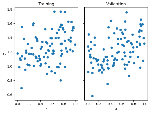

Now we can start fitting our model using our implemented LinearRegression class. We first test out our fit_analytic function.

from linear_regression import LinearRegression

LR = LinearRegression()
LR.fit_analytic(X_train, y_train)

print(f"Training score = {LR.score(pad(X_train), y_train).round(4)}")
print(f"Validation score = {LR.score(pad(X_val), y_val).round(4)}")

Training score = 0.1464
Validation score = 0.1548

When we inspect our training and validation scores, we see that they may not be as high as the scores we would get on classification models in the past. This is because it all depends on the randomly generated data we get and how much noise is present in it. We can also inspect its estimated weight vector as shown below.

LR.w

array([0.31040324, 1.0968243 ])

Next, we try testing out our fit_gradient function, and inspect its weight.

LR2 = LinearRegression()

LR2.fit_gradient(X_train, y_train, alpha = 0.01, max_iter = 1e3)

LR2.w

array([0.31041385, 1.09681821])

We see that its weight is pretty close to the weight calculated in our fit_analytic function. Since our fit_analytic keeps track of the scores of the current weight, we can also inspect its score_history.

plt.plot(LR2.score_history)
labels = plt.gca().set(xlabel = "Iteration", ylabel = "Score")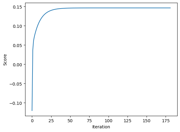

As expected, we see the score increases monotonically in each iteration.

Based on this demo, it looks like our LinearRegression class is working adequately.

Linear Regression Experiments

Next, we want to explore what overparameterization can do to our model. To do so, we run an experiment where we increase p_features, the number of features used, but keep n_train, the number of training points, constant. We do this until p_features is all the way to n_train - 1 and inspect their change in training and validation scores.

n_train = 100
n_val = 100
p_features = 1
noise = 0.2

training_scores = []
validation_scores = []

while (p_features < n_train):
    # create some data
    X_train, y_train, X_val, y_val = LR_data(n_train, n_val, p_features, noise)
    LR = LinearRegression()
    LR.fit_analytic(X_train, y_train)
    training_scores.append(LR.score(pad(X_train), y_train))
    validation_scores.append(LR.score(pad(X_val), y_val))
    p_features += 1
    
plt.plot(training_scores, label="training")
plt.plot(validation_scores, label="validation")

plt.xscale('log')
legend = plt.legend() 
labels = plt.gca().set(xlabel = "Number of Features", ylabel = "Score")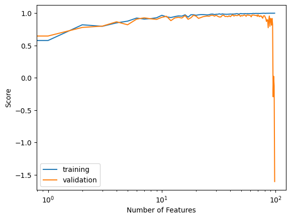

When we inspect our evolution of training scores, we see that generally as our number of features increases, our training score also increases and eventually reaches a perfect training score. When we inspect our evolution of validation scores, however, we see that as our number of features increases, our validation score decreases and eventually shoots down to a very low validation score.

This evolution of the training and validation scores follows the pattern of overfitting. Here, as the number of features increase, we see a gap between the training and validation score get larger. Perhaps this tells us that the more features we use with least squares linear regression the more vulnerable we are to overfitting.

LASSO Regularization Experiments

Let’s try the same experiment with the LASSO algorithm as provided through the sklearn.linear_model. This algorithm has a modified loss function with a regularization term, which makes the entries of the weight vector \(\mathbf{w}\) small. LASSO tends to force entries of the weight vector to be exactly zero, which may be desirable in our experiments where we are increasing the number of features to the number of data points.

We first experiment with our regularization strength set to \({\alpha} = 0.01\).

from sklearn.linear_model import Lasso

n_train = 100
n_val = 100
p_features = 1
noise = 0.2

training_scores = []
validation_scores = []

while (p_features < n_train):
    L = Lasso(alpha = 0.01)
    # create some data
    X_train, y_train, X_val, y_val = LR_data(n_train, n_val, p_features, noise)
    L.fit(X_train, y_train)
    training_scores.append(L.score(X_train, y_train))
    validation_scores.append(L.score(X_val, y_val))
    p_features += 1
    
plt.plot(training_scores, label="training")
plt.plot(validation_scores, label="validation")

plt.xscale('log')
legend = plt.legend() 
labels = plt.gca().set(xlabel = "Number of Features", ylabel = "Score")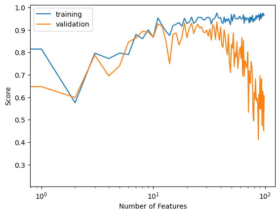

Here we see that as our number of features increased, our training score still increased to a close to perfect score, but our validation score is not as low as it was in least squares linear regression and the gap between these two scores is no longer as wide.

Now let’s strengthen our regularization to \({\alpha} = 0.1\).

n_train = 100
n_val = 100
p_features = 1
noise = 0.2

training_scores = []
validation_scores = []

while (p_features < n_train):
    L = Lasso(alpha = 0.1)
    # create some data
    X_train, y_train, X_val, y_val = LR_data(n_train, n_val, p_features, noise)
    L.fit(X_train, y_train)
    training_scores.append(L.score(X_train, y_train))
    validation_scores.append(L.score(X_val, y_val))
    p_features += 1
    
plt.plot(training_scores, label="training")
plt.plot(validation_scores, label="validation")

plt.xscale('log')
legend = plt.legend() 
labels = plt.gca().set(xlabel = "Number of Features", ylabel = "Score")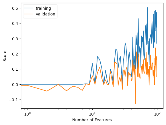

Here, when our regularization is set to an even higher value, we see the gap between our training and validation score get even smaller as our number of features increase.

Let’s now see how the LASSO algorithm with a high regularization term can handle when our number of features goes past the number of data points we have.

n_train = 100
n_val = 100
p_features = 1
noise = 0.2

training_scores = []
validation_scores = []

while (p_features < n_train + 100):
    L = Lasso(alpha = 0.1)
    # create some data
    X_train, y_train, X_val, y_val = LR_data(n_train, n_val, p_features, noise)
    L.fit(X_train, y_train)
    training_scores.append(L.score(X_train, y_train))
    validation_scores.append(L.score(X_val, y_val))
    p_features += 1
    
plt.plot(training_scores, label="training")
plt.plot(validation_scores, label="validation")

plt.xscale('log')
legend = plt.legend() 
labels = plt.gca().set(xlabel = "Number of Features", ylabel = "Score")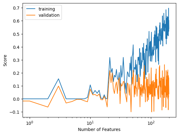

Based on our graph of scores, we see that the validation score fluctuates a little, but generally stays within the same range even as our number of features exceed our number of data points.

As we see through these experiments, the LASSO algorithm, when provided with a strong regularization term, can handle overparameterization better than our least square linear regression model.