Composer Classification
Abstract
The aim of this project was to develop a machine learning model capable of differentiating the compositions of a classical music composer. Specifically, our focus centered on determining whether or not a given piece of classical music was composed by Beethoven. The MusicNet data set, consisting of 330 .wav files, served as the primary data source for training and evaluation. Convolutional Neural Network (CNN) models and Recurrent Neural Network (RNN) models were developed and trained using appropriate preprocessing techniques and feature extraction methods. The RNN models achieved an average accuracy rate of 76%, while the CNN models achieved an average accuracy rate of 74%. While the achieved accuracies fell below the desired results, this project provided valuable insights into the challenges of attributing classical music compositions.
GitHub Repository: MLProject
Introduction
When listening to music, it’s common to encounter an unfamiliar song that one wishes to quickly identify. To address this challenge, our project leverages the MusicNet data set to classify whether a given piece of classical music is composed by Beethoven. This project aimed to tackle this seemingly small but persistent issue, with the hope of contributing to the larger music identification problem.
There is a limited number of resources on how researchers within the Machine Learning field addressed this problem. On the other hand, genre classification using music audio files is a widely explored problem with numerous approaches available. Costa, Oliveira, and Silla Jr (2017) used the ISMIR 2004 Database, the LMD database, and a collection of field recordings of ethnic African music to train a model to classify music genres. They found that the spectrograms of audio when used with a CNN model performs just as well if not better than individual classifiers trained with visual representation on all datasets. Khamees et al. (2021) used the GTZAN data set for music classification. In their studies, they created and compared the performance of CNN and RNN models. They found that a CNN model with Max-Pooling outperformed RNN with LSTM. The CNN model yielded a testing accuracy of 74% and the RNN model yielded a testing accuracy of 63%. Kakarla et al. (2022) also used the GTZAN dataset, worked with the MFCCs of audio files, and found that a 5-layered independent RNN was able to achieve 84% accuracy.
While our project may not be as complex as music genre classification, we used this research as guidance and created a variety of simple CNN models and RNN models with LSTM to work towards this problem of identifying the composer of classical music.
Values Statement
As avid music listeners, we were drawn to the idea of creating a project focused on analyzing music using its audio files. Our project could potentially be used by music theory researchers, classical music listeners, and anyone interested in exploring this genre. If we kept the labels indicating the original composer rather than changing it to “Other,” we could potentially identify patterns and influences among different composers. It’s also important to note that our models were only trained on classical music from Western composers, potentially perpetuating inequalities in the music industry. Misclassifications could also result in the improper attribution of credit to certain composers. While our project is still small in scale, we recognize that as it grows, it may require additional computational resources, which could introduce environmental concerns.
While our project can do a better job of incorporating classical music from non-Western composers, we still believe that it could bring joy and value to the world of classical music.
Materials and Methods
Data
We utilized the MusicNet data set, which encompassed a collection of 330 audio files of classical music. These files have varying durations with the shortest being 55 seconds and longest being almost 18 minutes. Approximately 48% of the data set consisted of pieces composed by Beethoven, while the remaining files were by other composers. The audio files also exhibited a diverse range of instruments.
Approach
To ensure a fair comparison of the models’ ability to distinguish Beethoven’s music, we standardized the data set by using only the first 45 seconds of each audio file. Furthermore, we divided this 45 seconds segment into 15 smaller pieces, each lasting 3 seconds. This subdivision allowed us to generate additional data points, which was beneficial for training and evaluating our neural network models.
After segmenting the audio files, we obtained a total of 4950 pieces of data. To ensure an effective training process, we split the data using an 80-20 ratio. Specifically, 80% of the data was allocated for training purposes, while the remaining was reserved for testing the models’ performance. Within the training data, we further divided it into an 80-20 ratio, designating 80% for training and 20% for validation.
To evaluate the performance of our models during training and validation phases, we tracked the history of loss and accuracy metrics. Given the large storage requirements of audio files, we conducted our work primarily on Google Colab.
CNN
The CNN models we developed utilized mel spectrograms, which are visual representations of audio data, as the input features. Mel spectrograms, also known as Mel-frequency spectrograms, share a similar structure to regular spectrograms, featuring a two-dimensional image format where the x-axis represents time and the y-axis represents frequency. The intensity represented by the color of each point in the mel spectrogram image corresponds to the magnitude of the associated frequency component. Notably, mel spectrograms differ from regular spectrograms in that they apply a frequency warping known as mel scale, aligning the frequency representation to better match human auditory perception. For our targets, we used our composer labels. Given the straightforward nature of our task, we proceeded to train two versions of our model, which consisted of six convolutional layers followed by a max-pooling layer. The two variations included one model with a dropout layer and another model without it.
RNN
Another model we used to analyze our clips of music was a recursive neural network (RNN) with long short-term memory (LSTM), which is good at understanding order and analyzing sequential data. We utilized the mel-frequency cepstral coefficients (MFCC) of our audio clips as the input features. MFCCs are commonly used frequency domain features that represent the frequencies perceived by the human ear and capture the “brightness” of sound. For this model, we also used our composer labels as targets. Since our task was fairly simple, we trained four variations of LSTM models. We first experimented with 1 LSTM layer and 2 LSTM layers. Then to prevent overfitting, we experimented with 1 LSTM layer with a dropout layer and 2 LSTM layers with a dropout layer, both with a of probability of 0.2.
Results
CNN
Below are the history of our training and validation accuracy for the CNN models with and without a dropout layer.
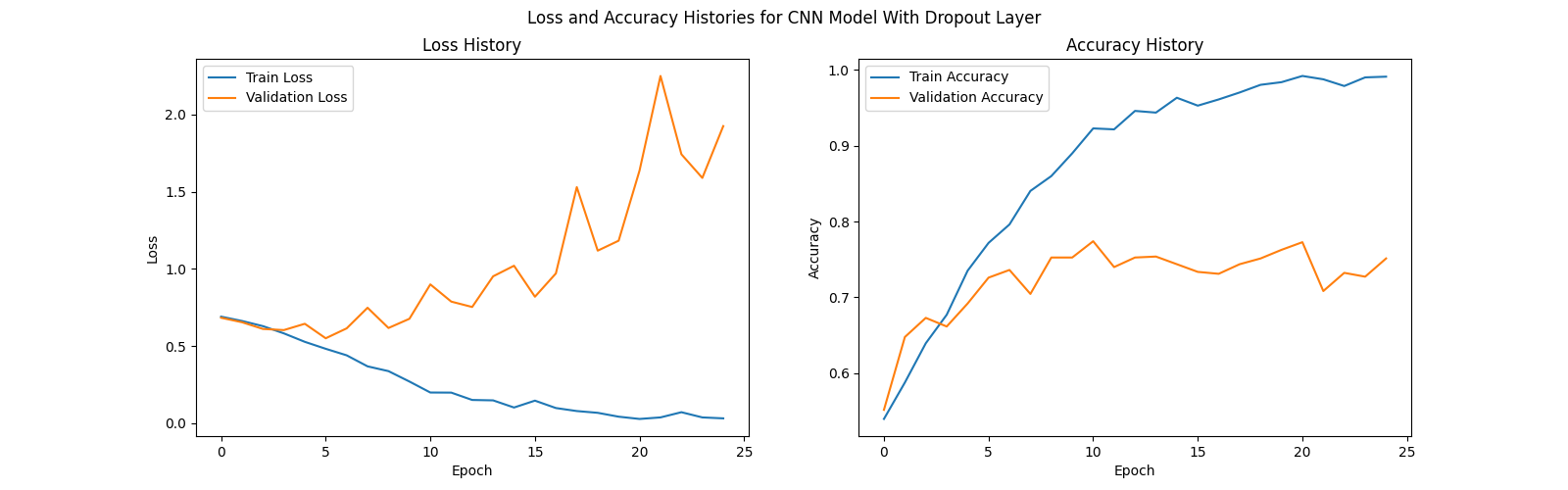
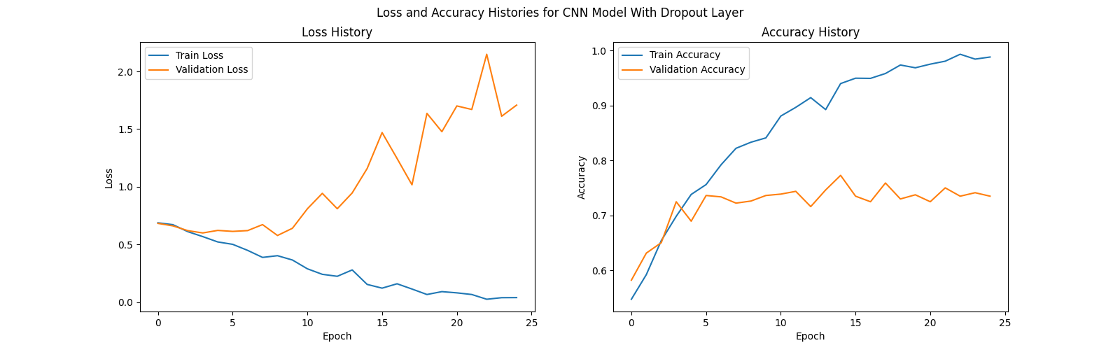
For each of our CNN models, we trained for a total of 25 epochs. Despite using a dropout layer (probability = 0.2), both models still showed signs of significant overfitting. The model without the dropout layer yielded a testing accuracy of 74%, while the model with the dropout later yielded a testing accuracy of 73%.
RNN
Below are the history of our training and validation accuracy for our RNN models with 1 LSTM layer, 2 LSTM layers, 1 LSTM layer and a dropout layer, and 2 LSTM layers and a dropout layer.
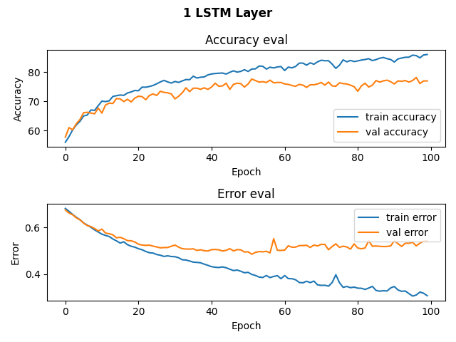
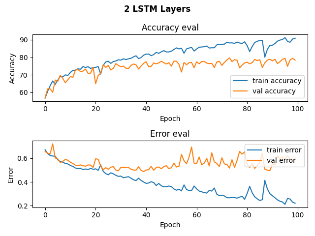
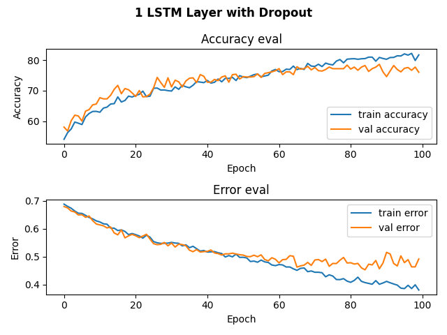
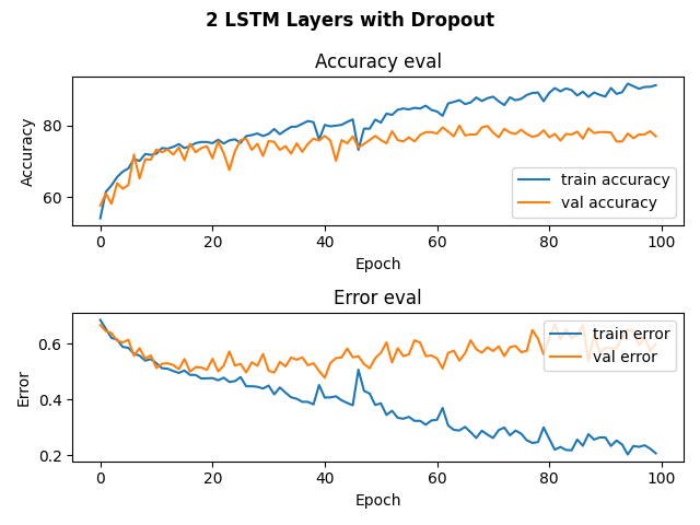
As conveyed in the graphs, we trained for about 100 epochs, for that’s when it looked like the training validation accuracy started to plateau and were never able to surpass a training validation accuracy of 80%. For our model with 1 LSTM layer, we achieved a testing accuracy of 74%. For our model with 2 LSTM layers, we achieved a testing accuracy of 78%. For our models with dropout layers, we achieved a testing accuracy of 76%. While these accuracies are not the best, they are better than randomly guessing given that 48% of our data is Beethoven.
We would also like to acknowledge that our results are based on one round of training on our data. In order to achieve more accurate results, we understand that training our models multiple times and averaging their results would provide a more accurate representation of how our models do.
Concluding Discussion
In conclusion, our CNN models and RNN models were able to classify whether a piece of classical music was composed by Beethoven with an average testing accuracy of 75%. Although we weren’t able to reach our goal of an 80-85% testing accuracy, our results are still higher than our base rate of 48%. Since there aren’t many studies on composer classification, we referenced studies on music genre classifications. Our models produced similar testing accuracy compared to those studies.
If we had more time, we would’ve been more mindful of how we cleaned our data. We spent a lot of time just trying to understand how processing and extracting features from audio data works. By the time that we finished cleaning our data, we weren’t fully aware of the complications that multiple instruments and segments of rests could introduce. In addition, we would’ve segmented the entirety of each piece, which would’ve resulted in more data points. We also would’ve spent more time fine tuning our models and playing with different variations.
Group Contribution Statement
The work for this project was fairly evenly distributed.
Vy Diep wrote the code for the data relabeling and organization. She also developed the CNN model training and experimentation. For our presentation, she led the discussion on our approach and CNN results. For the blog post, she led the writing for the Abstract, Data, Approach, and CNN results sections.
Katie Macalintal wrote the code for the RNN model training and experimentation. For our presentation, she led the discussion on the overview of our project and RNN results. For the blog post, she led the writing for the Introduction, Values Statement, and RNN results sections.
There were also a handful of tasks that Katie and Vy would do together, but only one person would commit. We would often clean up our GitHub repository together and for the blog post, we worked together to craft the concluding discussion.
Personal Reflection
This project has taught me a lot about the process of researching, implementing, and communicating. It has introduced me to the challenges of working with big data, showed me the importance of hardware choices, and strengthened my skills with creating training loops and using PyTorch. While I am proud that our models were close to reaching our goals of 80-85% testing accuracy and that my partner and I were able to work collaboratively throughout this project, I do think that there are a handful of things we could have done better.
I think that we definitely could have spent more time researching. Going into this project, we felt a sense of urgency in making models right away out of fear that we would run out of time for training. This definitely affected our mindset throughout this project, for I feel like we did not spend enough time researching or thoroughly understanding the implications of different audio elements. Throughout the course of this project, we would often go through this cycle of reading only one or two articles and then implementing what they did. However, we would then read another article or two, learn more about a more efficient approach, but not have enough time to modify the way in which we prepped our data. Since my partner and I each focused on a developing different models and didn’t really work in the same files, our conventions for code cleanliness and format differed. If we had not rushed and instead completed most of our research before implementing, I think that we would have prepared our data in a cleaner way that was uniform across both models.
Overall, I’m somewhat satisfied with this project, but definitely think that it could have gone better. When I do my next project, whether it is related to machine learning or not, I will work to do more research before implementing, continue to be a collaborative and responsive teammate, and be thoughtful about who it can harm and who it can help.